Risk Professionals: Build Regulator Ready PD, LGD, and EAD Models

Probability of default (PD) measures the likelihood a borrower fails to repay within a defined period. Loss given default (LGD) is the share of exposure a lender loses after recoveries, expressed as a fraction. Exposure at default (EAD) is the dollar amount outstanding when default happens. Multiply the three together, PD × LGD × EAD, and you get expected loss (EL). IFRS 9 complicates the picture by requiring a 12-month PD for performing loans and a lifetime PD once credit quality deteriorates.

---

TL;DR:

• Basel’s regulatory models favor through-the-cycle PD estimates for capital, while IFRS 9 requires point-in-time PDs that incorporate current macroeconomic conditions.
• Modeling EAD on revolving facilities must include undrawn commitments and accurate CCF assumptions, validated against actual drawdown behavior.
• During downturns, PD, LGD, and EAD tend to increase simultaneously, and ignoring their joint behavior can significantly underestimate tail risk.
• Ensuring consistency in default definitions across PD and LGD models is critical, as misalignment can undermine model validation and expected loss accuracy.
• Incorporating macroeconomic scenario overlays and joint dependence models improves stress testing accuracy and aligns with most regulatory expectations.

---

Table of Contents

• Understanding PD LGD EAD Definitions and a Worked Example
• Basel IRB and IFRS 9: Two Different Jobs for the Same Inputs
• How Do You Build and Validate a PD Model?
• Why Do LGD Models Need a Two-Stage Approach?
• Estimating EAD: CCFs and Undrawn Exposure
• Why Do PD, LGD, and EAD Move Together in a Downturn?
• What Data and ML Practices Belong in a PD LGD EAD Framework?
• Practitioner Checklist for PD LGD EAD Governance
• How Basel II/III Uses PD, LGD, and EAD for Capital Requirements
• How Macroeconomic Conditions Change PD, LGD, and EAD Estimates
• Why Does the Default Definition Change PD and LGD Estimates?
• Ready to Put PD, LGD, and EAD Into Practice?
• The Next Two Years of PD, LGD, and EAD Modeling
• Sources
• FAQ

Understanding PD LGD EAD Definitions and a Worked Example

Each of these three inputs uses a different unit, and mixing them up is the single most common error analysts make when building an expected loss model. PD is a probability between 0 and 1, always tied to a time horizon, such as “1.8% over 12 months.” LGD is also a fraction between 0 and 1, representing the portion of exposure the lender does not recover after collateral sale, workout costs, and time value are accounted for. EAD is a dollar figure, the balance outstanding (or expected to be outstanding) at the moment of default.

Here’s a simple example using round numbers:

1. A commercial loan has an EAD of $500,000 at the point of default.
2. The lender estimates LGD at 40%, meaning it expects to lose $200,000 net of recoveries.
3. The borrower’s 12-month PD is 2%.
4. Expected loss = 0.02 × 0.40 × $500,000 = $4,000.

That $4,000 figure is the loan’s 12-month expected credit loss (ECL) under IFRS 9 Stage 1. If the loan migrates to Stage 2 because credit risk has increased significantly, the calculation switches to a lifetime PD, which is typically much higher than the 12-month figure and must be discounted back to present value using the loan’s effective interest rate, as outlined in IFRS 9 practitioner guidance on ECL calculation. A frequent mistake: using a drawn-balance-only EAD on a revolving facility when the undrawn portion also carries default risk.

Basel IRB and IFRS 9: Two Different Jobs for the Same Inputs

PD, LGD, and EAD serve two separate regulatory purposes, and confusing them creates real audit exposure. Basel’s Internal Ratings-Based (IRB) approach uses these three inputs to calculate regulatory capital, generally favoring through-the-cycle (TTC) PD estimates that smooth out short-term volatility, per the Basel Framework published by the BIS. IFRS 9 uses the same three inputs for loan-loss provisioning, but it demands point-in-time (PIT) PD estimates that reflect current and forecast economic conditions, weighted across multiple macroeconomic scenarios.

That difference in philosophy, TTC for capital stability versus PIT for provisioning accuracy, is where most model governance headaches start. Regulators and auditors tend to flag the same handful of issues repeatedly:

• Overlays applied to model outputs without a documented rationale or approval trail
• Downturn LGD estimates that rely on benign historical periods instead of stressed vintages
• Credit conversion factor (CCF) assumptions with thin or unrepresentative evidence for undrawn exposures
• Inconsistent default definitions between the PD model’s training data and the LGD model’s loss population
• Missing reconciliation between modeled LGD and actual settled losses over time

Supervisory guidance on stress-test methodology, including the Federal Reserve’s descriptions of supervisory models, makes clear that examiners expect operational controls, not just strong backtest numbers.

How Do You Build and Validate a PD Model?

PD modeling starts with picking the right technique for the portfolio and the data available. Logistic regression scorecards remain the industry default because they’re transparent and easy to validate. Survival analysis works better when you need a full term structure of marginal PDs rather than a single point estimate. Machine learning classifiers (gradient boosting, random forests) can improve discrimination on large, feature-rich portfolios, but they demand more explainability work to satisfy auditors, a tension well documented in research on ML adoption and explainability in credit risk.

Building a term structure means generating marginal, year-by-year PDs rather than a flat lifetime average, then converting a TTC baseline to a PIT estimate using macroeconomic overlays tied to unemployment, GDP growth, or housing price indices.

Validation is not optional and it is not a one-time event. At minimum, run these tests on a regular cycle:

• Discrimination: AUC or Gini coefficient, checked against a documented minimum threshold
• Calibration: predicted PD versus observed default rate, by score band and in aggregate
• Population Stability Index (PSI): tracks whether the scored population still resembles the development sample
• Out-of-time holdouts and rolling backtests to confirm the model still performs on recent vintages

Pro Tip: An open-source mortgage credit risk model on GitHub demonstrates that well-calibrated PD models can reach an AUC around 0.8 on clean data. Treat that figure as a sanity check, not a universal benchmark. Every portfolio’s ceiling depends on data quality and default rarity.

Why Do LGD Models Need a Two-Stage Approach?

LGD estimation gets messy fast because many defaulted accounts recover in full, and a single regression line can’t handle that reality well. The industry’s standard fix is a two-stage, or hurdle, model: a logistic regression first predicts the probability that a loss occurs at all, then a separate model estimates severity conditional on a loss actually happening. This structure is more robust than a single linear model whenever the defaulted-loan population includes a meaningful share of zero-loss outcomes.

Recovery estimation itself depends on several moving parts:

• Collateral valuation at the point of default, updated for market conditions rather than origination-date values
• Enforcement and liquidation costs, including legal fees, holding costs, and broker commissions
• Time-value discounting, since recoveries on defaulted commercial real estate can take 18 to 36 months to materialize

Downturn LGD adds a further layer: Basel and IFRS 9 both expect loss severity assumptions to reflect stressed conditions, not benign historical averages, since collateral values and recovery timelines both worsen in a downturn. Document the haircut methodology explicitly, showing the link between the stress scenario chosen and the historical or hypothetical loss data that supports it.

Pro Tip: Reconcile every modeled LGD estimate against settled-loss records at least annually, and cap outlier recoveries so a handful of unusually strong workouts don’t understate your downturn assumption.

Estimating EAD: CCFs and Undrawn Exposure

EAD calculation is straightforward for a fully drawn term loan (it’s just the outstanding balance) and considerably harder for revolving credit lines, where borrowers can draw down more of their commitment as they approach default.

1. Start with the drawn balance at the reporting date.
2. Add the undrawn commitment multiplied by a Credit Conversion Factor (CCF), a percentage that estimates how much of the unused line gets drawn before default.
3. Segment CCF estimates by product type and borrower risk grade, since a distressed borrower typically draws down a revolving line far more aggressively than a healthy one.
4. Validate CCF assumptions against realized drawdown behavior in your own default history, not industry averages alone.

Behavioral evidence consistently shows borrowers increase utilization of revolving facilities in the months before default, a pattern that term loans simply don’t exhibit. That’s why CCF estimation deserves its own dedicated data build rather than a borrowed rule of thumb.

Why Do PD, LGD, and EAD Move Together in a Downturn?

Treating PD, LGD, and EAD as independent inputs is a convenient simplification that breaks down exactly when it matters most: during stress. In a recession, default rates rise, collateral values fall (pushing LGD up), and distressed borrowers draw down more of their available credit (pushing EAD up) all at the same time. Modeling these three variables as if they move independently can significantly understate tail risk.

Research on modeling PD, LGD, and EAD jointly argues for treating EAD as stochastic rather than fixed, since correlations between the three inputs materially affect stressed loss and capital estimates. Practical techniques include:

• Factor models that link PD, LGD, and EAD to shared macroeconomic drivers
• Copula-based approaches to capture nonlinear dependence in the tails
• Scenario multipliers applied uniformly across a stress scenario to approximate joint deterioration
• Stochastic EAD simulation for revolving and commitment-heavy portfolios

Reflecting these joint shocks in capital and ECL computations, rather than applying stressed PD alone, tends to produce materially higher loss estimates. Institutions that skip this step often see backtest surprises the first time an actual downturn arrives.

What Data and ML Practices Belong in a PD LGD EAD Framework?

Core data requirements haven’t changed much in twenty years: default history with accurate timing, recovery and cash-flow records post-default, exposure histories showing drawdown behavior, and macroeconomic time series long enough to span at least one full credit cycle.

Alternative data is where the newer opportunity, and the newer risk, sits. Cash-flow patterns, rent payment history, and utility payment records can extend credit scoring to borrowers with thin traditional credit files. Federal research confirms this can expand credit access while requiring real privacy safeguards, including opt-in consent and Gramm-Leach-Bliley Act (GLBA) compliance.

• Confirm any alternative data source has documented consumer consent before it enters a model
• Test feature stability over time, since alternative data sources can shift structurally when a provider changes its methodology
• Maintain full documentation of every feature’s source, refresh cadence, and validation history for audit purposes

Pro Tip: If you adopt a machine learning classifier for PD, budget as much analyst time for explainability documentation (SHAP values, partial dependence plots, feature stability reports) as you spent building the model itself. Regulators will ask for it.

Practitioner Checklist for PD LGD EAD Governance

Auditors and regulators evaluate model quality and operational discipline together. Minimum documentation should include data lineage records, a written model specification, and full calibration and backtesting results tied to specific model versions.

1. Confirm discrimination and calibration metrics are refreshed on a defined schedule, not just at initial approval.
2. Run out-of-time performance checks before every annual model review.
3. Reconcile modeled LGD losses against settled-loss records and document any material variance.
4. Maintain a current model inventory with clear ownership and change-control logs.

• Published, transparent criteria (like advance-rate grids) reduce the ambiguity examiners flag most often in underwriting reviews.
• Fast, documented decisioning, closing in as little as four hours in CR Equity Ai Inc’s own underwriting process, illustrates how operational speed and audit-ready documentation can coexist rather than trade off against each other.

How Basel II/III Uses PD, LGD, and EAD for Capital Requirements

Under the IRB approach, PD, LGD, and EAD feed directly into the risk-weighted asset (RWA) formula, which then determines how much regulatory capital a bank must hold against a given exposure. The Basel Framework sets the underlying risk-weight functions, but the intuition is straightforward: higher PD, higher LGD, and higher EAD each independently push RWA up, and therefore push the required capital buffer up.

Consider a simplified illustration. A $1 million commercial real estate loan with a 1.5% PD and a 35% LGD generates a lower risk weight than an otherwise identical loan with a 4% PD and the same LGD. The capital charge scales with that risk weight, meaning a loan book skewed toward higher-PD borrowers requires meaningfully more capital to support the same total lending volume, even if the average loan size is identical.

Basel III layered additional constraints on top of the original IRB framework, including capital floors that limit how far a bank’s internal models can reduce RWA relative to the standardized approach. This matters directly for PD, LGD, and EAD model design: even a highly accurate internal model won’t help much if the floor binds. Institutions building or recalibrating IRB models should test both the modeled RWA outcome and the floor-constrained outcome, since supervisors increasingly focus review time on cases where the two diverge significantly.

Downturn LGD carries particular weight in this calculation because Basel requires it specifically for capital purposes, not just for IFRS 9 provisioning. A bank that uses benign-period LGD assumptions in its capital calculation risks materially understating the capital it needs to hold through a full credit cycle, a gap that tends to surface exactly when reserves are needed most.

How Macroeconomic Conditions Change PD, LGD, and EAD Estimates

Macroeconomic conditions don’t just add noise to PD, LGD, and EAD estimates. They drive the direction and magnitude of all three simultaneously, which is why static, unconditional models tend to underperform right when accuracy matters most.

Unemployment rate changes correlate closely with PD across most consumer and small-business portfolios, while GDP growth and industry-specific indicators tend to matter more for commercial and CRE exposures. When unemployment rises or a specific property sector softens, default rates climb with a lag of roughly two to four quarters in many portfolios, which is why IFRS 9’s probability-weighted, multi-scenario approach exists in the first place: a single-point forecast misses the shape of that lag entirely.

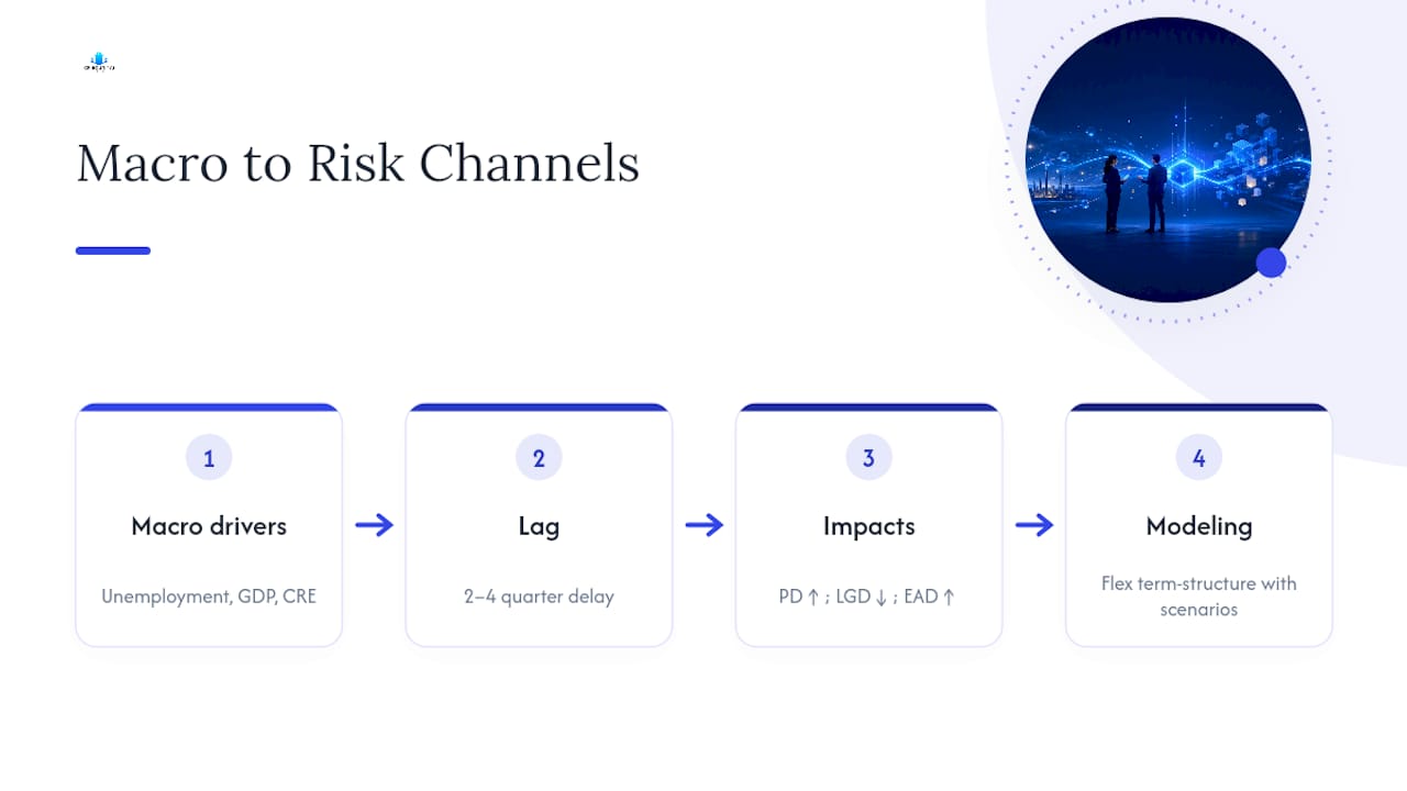
LGD responds to macro conditions primarily through collateral values. Falling commercial real estate prices during a downturn directly reduce recovery amounts, while extended enforcement timelines in a stressed market increase the time-value discount applied to eventual recoveries. This is the core justification for downturn LGD add-ons under both Basel and IFRS 9.

EAD responds differently: distressed borrowers draw down revolving facilities more heavily as conditions worsen, meaning CCF assumptions calibrated on a benign period will understate exposure exactly when losses are rising. Building CCF and PD term-structure models that both flex with macro scenario inputs, rather than treating macro sensitivity as a bolt-on overlay, produces more defensible stress and ECL outputs. Institutions that model macro sensitivity only in PD, and hold LGD and EAD static, are the ones most likely to see stressed loss forecasts miss badly in an actual downturn.

Why Does the Default Definition Change PD and LGD Estimates?

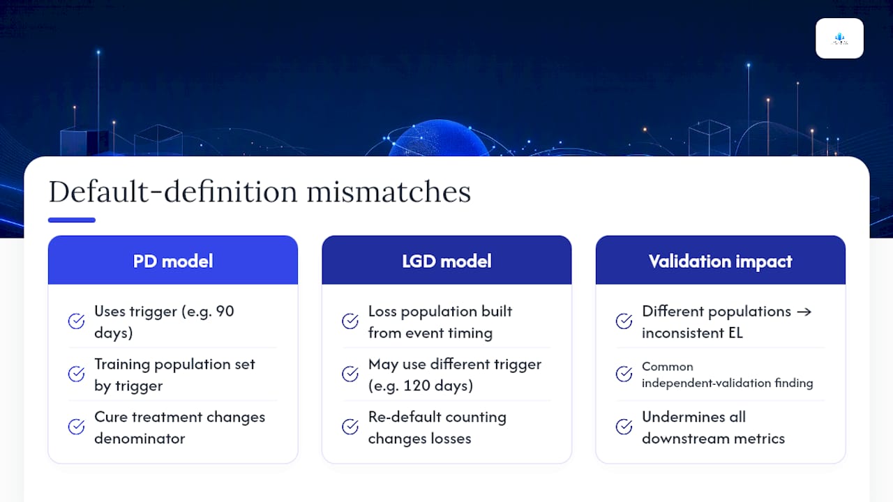
The default definition a bank uses shapes every downstream PD and LGD number, which makes it one of the highest-leverage governance decisions in the entire modeling framework. Basel’s standard default definition combines a 90-days-past-due trigger with unlikeliness-to-pay indicators, but banks retain some discretion in how they operationalize “unlikely to pay,” and that discretion creates real inconsistency risk across a model suite.

Timing matters just as much as the trigger itself. If a PD model’s training data uses a 90-day trigger but the LGD model’s loss population was built from accounts that entered workout at 120 days, the two models are effectively measuring different populations, and expected loss calculations built on top of them will be internally inconsistent. This is one of the most common technical findings in independent model validation reviews.

Cure and re-default treatment adds another layer of complexity. A borrower who goes 95 days past due, cures, then re-defaults eight months later needs a documented, consistently applied rule for whether that counts as one default event or two, since it directly affects both the PD denominator and the LGD loss population.

Getting default definitions aligned across the PD model, the LGD model, and the loss data used to validate both isn’t a compliance afterthought. It’s the foundation the entire expected loss calculation rests on, and misalignment here quietly undermines every validation metric built downstream, no matter how sophisticated the modeling technique.

Ready to Put PD, LGD, and EAD Into Practice?

Model theory only proves its worth when it survives contact with a real underwriting decision. CR Equity Ai Inc underwrites the asset and the deal itself, not just borrower paperwork, using a soft credit pull and decisions in as little as four hours on most real estate programs, an approach that puts many of the documentation and speed principles covered above into daily practice. If you’re evaluating financing for an acquisition, a fix-and-flip project, or a ground-up build and want to see how disciplined underwriting translates into a real quote, you can request a loan quote directly and see program terms firsthand.

The Next Two Years of PD, LGD, and EAD Modeling

Machine learning will keep gaining ground in PD modeling, but not unconditionally. The institutions getting this right pair ML gains with genuine explainability tooling rather than treating documentation as an afterthought bolted on before an exam. My honest read: the teams that win the next cycle won’t be the ones with the fanciest model architecture. They’ll be the ones who invested early in data quality, built scenario governance that regulators can actually follow, and stayed in dialogue with examiners instead of surprising them at review time.

— Robert

This article is general information, not a substitute for advice from a qualified financial advisor. Consult a qualified financial professional about your own circumstances before acting on anything here.

Sources

• The Fed — Descriptions of supervisory models
• CRS product: Alternative Data in Financial Services (IF11630)

FAQ

Recommended

• Examples of Credit Risk Models for Risk Professionals
• Loan Scenario Analysis Best Practices for Credit Officers